Ray casting in 2D game engines

Introduction

In my opinion, ray casting is a beautiful concept that is not that hard to grasp, but the quality resources are rare. We will learn the math behind it so you can implement it in your future projects with ease. I will try to make it as comprehensible as possible, explain all the caveats and issues you may stumble upon. We will also talk about optimization and how can spatial hash maps significantly help you. I will also provide some basic live examples for you to try out. Please note that demos were written to be as simple as possible, do not expect enterprise-grade code - we only learn about the concept, not the implementation.

What is ray casting?

Ray casting is the most basic of many computer graphics rendering algorithms that use the geometric algorithm of ray tracing. Ray tracing-based rendering algorithms operate in image order to render three-dimensional scenes to two-dimensional images... The idea behind ray casting is to trace rays from the eye, one per pixel, and find the closest object blocking the path of that ray – think of an image as a screen-door, with each square in the screen being a pixel. This is then the object the eye sees through that pixel.

Well, it does not tell us much, does it? Let me simplify that. Ray casting is a fundamental and popular technique used to determine the visibility of specific objects (polygons) by tracing rays from the eye (for instance, player’s hero) on every pixel (well, not quite in our case - more on that later) and finding the nearest intersections with objects.

Where might ray casting be used?

Ray casting has many uses, especially in three-dimensional space. I outlined three, in my opinion, the most important, which are commonly used in 2D game engines:

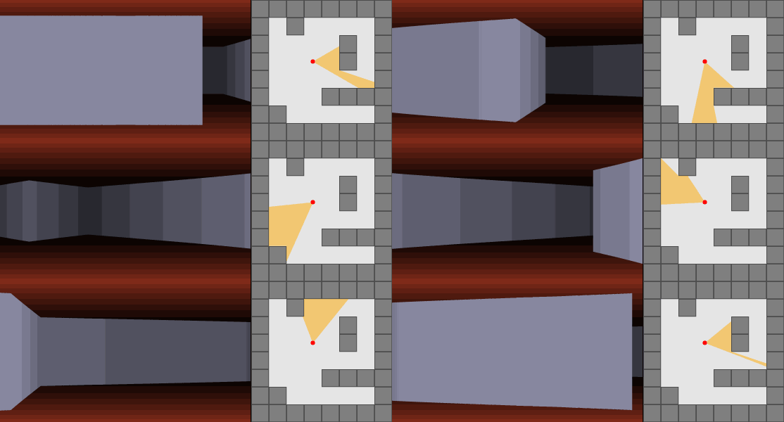
Creating 3D perspective in a 2D map

The most well-known game that used this technique is Wolfenstein 3D. Rays were traced to determine the closest objects, and their distance from the player position was used to appropriately scale them.

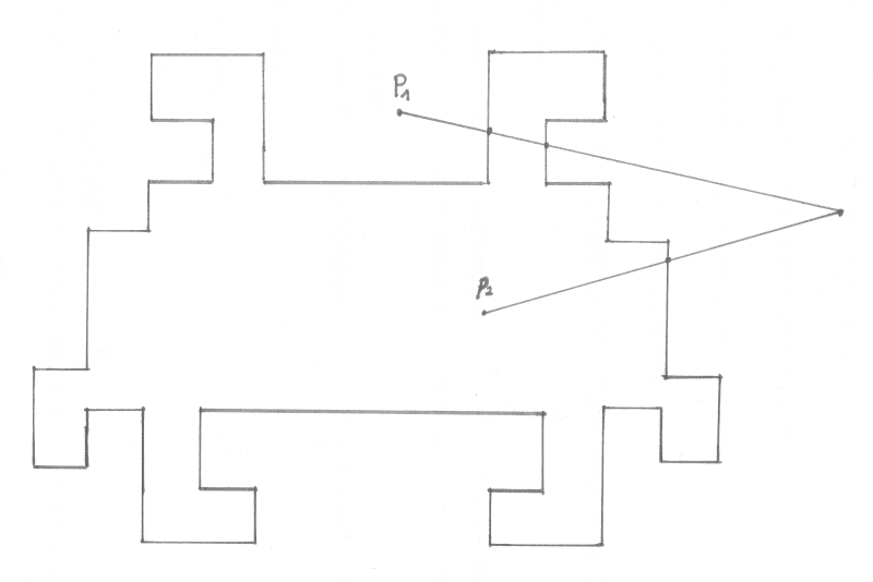
Point-in-polygon problem

PIP problem asks whether a given point lies inside, outside, or on the boundary of a polygon. Using the ray casting algorithm, we can count how many times the point intersects the edges of the polygon. If the number of the intersections is even, the point is on the outside of the polygon. If the number of the intersections is odd, the point is on the inside or on the boundary of a polygon.

Object visibility and light casting

This is the problem we will specifically tackle in this article - determining which objects are visible by the player and illuminating the visible area.

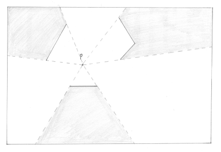
Object visibility and light casting in 2D games

In this section we will go through basics such as calculating intersection points, casting rays, sorting intersection points to illuminate the visible area, and few words about circles. I will provide interactive demos at each stage so you do not get lost and see the results immediately.

Line-segment - ray intersection point

It is all about those intersection points. Let's learn step by step how to find them and how to use them. We will derive a line parametric equation first, calculate intersection points and finally learn how to determine which one of them is the closest efficiently.

Deriving line parametric equation

Let us talk about lines and their parametric equation first.

We can express vector \(\overrightarrow{AP}\) by the following equation: \(\overrightarrow{AP} = t\overrightarrow{AB}\), where \(t\) is an equation parameter defining how much do we stretch (\(|t| > 1\)) or shrink (\(|t| < 1\)) and if we flip the direction (\(t < 0\)) of vector \(\overrightarrow{AP}\) in relation to vector \(\overrightarrow{AB}\).

Let me show you few examples:

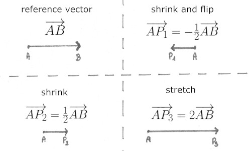
As you might have noticed, we can use \(t\) as a scale factor: \(|AP| = |t||AB|\). We will use that fact when determining the closest intersection point.

Now we can easily see, that if we want the point to be contained on:

• line: \(t \in \mathbb{R}\),
• ray: \(t \geq 0\),
• line-segment: \(0 \leq t \leq 1\).

Having all of that sorted out, we can finally derive the parametric equation:
\[ \begin{align} \overrightarrow{AP} &= t \overrightarrow{AB} \\ P - A &= t (B - A) \\ P &= t(B - A) + A \\ \end{align} \]

If you still do not know what happens here, I can recommend an awesome short lecture by Norm Prokup: Parametrizing a Line Segment - Concept.

Calculating the intersection point

Assume that point \(P\) is the intersection point of line-segment defined by points \(A\) and \(B\), and ray defined by points \(C\) and \(D\). Point \(P\) is then expressed by set of two equations: \[ \left\{\begin{align} P &= s(B - A) + A\text {, where } 0 \leq s \leq 1 \text{, and} \\ P &= r(D - C) + C\text {, where } r \geq 0 \text{.} \end{align}\right. \]

Solve for \(s\) and \(r\): \[ \left\{\begin{align} s(B_x - A_x) + A_x &= r(D_x - C_x) + C_x \Rightarrow s = \tfrac{r(D_x - C_x) + (C_x - A_x)}{B_x - A_x} \\ s(B_y - A_y) + A_y &= r(D_y - C_y) + C_y \Rightarrow r = \tfrac{s(B_y - A_y) + (A_y - C_y)}{D_y - C_y} \end{align}\right. \]

Having \(s\) and \(r\) calculated, we can calculate \(P\) using one of the equations from the set.

Finding the closest intersection point

We only need the closest intersection point to properly draw the visible area. The naive solution would be to calculate distances between the ray starting point and intersection points using the Pythagorean Theorem: \(\sqrt{(C_x - P_x) ^ 2 + (C_y - P_y) ^ 2}\). Remember the line equation parameter, though? I have already mentioned that we can use it as a scale factor. As we want to compare distances on ray, we can check for the smallest \(r\) parameter value: \(|\overrightarrow{CP_1}| < |\overrightarrow{CP_2}| \Leftrightarrow |r_1| < |r_2|\).

Casting rays

In the following section we will go through two different ways rays might be cast. We will compare them and mention their pros and cons.

Casting rays by offset angle

First way is to cast rays in all directions by specified offset angle. For instance, we could cast 30 rays in total offseted by \(12^\circ\). Let's see how to generate all those rays first.

Let \(P_1 = (x_1, y_1)\) be an anchor point of our rays, and let \(P_2 = (x_2, y_2)\) be a some point on a line going through \(P_1\) at angle \(\phi\):

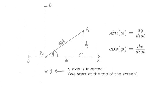
We can define \(x_2\) as \(x_1 + dx\) and \(y_2\) as \(y_1 - dy\) (our y-axis is inverted hence why the minus sign).
Now we need to derive formulas for \(dx\) and \(dy\): \[ \left\{\begin{align} \sin(\phi) &= \tfrac{dy}{\mathit{dist}} \Rightarrow dy = \mathit{dist} * \sin(\phi) \\ \cos(\phi) &= \tfrac{dx}{\mathit{dist}} \Rightarrow dx = \mathit{dist} * \cos(\phi) \end{align}\right. \] \(\mathit{dist}\) in our case has an arbitrary (greater than 0) value (we are looking for any point on the line), so we are safe to assume \(\mathit{dist} = 1\) to simplify the calculations. Having it all considered, \(P_2 = (x_1 + \sin(\phi), y_1 - \cos(\phi))\), where \(\phi\) is our angle offset.

Casting rays on vertices

Casting rays on vertices is most likely your go-to solution. Instead of casting rays in all directions, we can simply cast them on our polygons' vertices. Depending on the number of vertices, we can save computing power by not casting useless rays. In the next sections you will see how does it impact animation smoothness and also learn how to further optimize the whole process.

Illuminating the visible area

This is where the real fun begins. We will illuminate the visible area by filling a giant polygon.

Sorting intersection points

To correctly order vertices to build a proper polygon, we need to sort them by angle first. We will use \(atan2(y, x)\) function for that. You can read more about it here.

Let's compare both ray casting methods:

Both of them looks glitchy, jumpy and inaccurate. Let's take a closer look why.

Casting slightly offseted rays

Notice what happens when rays are cast directly on vertices - they should go beyond that vertex but we are getting only the closest intersection point:

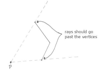
The most common solution is casting two extra rays offseted by small angle (in both directions) for every cast ray. Consider ray \(AB\) starting at \(A = (A_x, A_y)\) going through \(B = (B_x, B_y)\). We want to find such point \(C = (C_x, C_y)\) that ray \(AC\) would be rotated by \(\phi\) with \(A\) being the origin point. \(C\) coordinates would be as follow: \[ \left\{\begin{align} C_x &= (B_x - A_x)\cos(\phi) - (B_y - A_y)\sin(\phi) + A_x \\ C_y &= (B_y - A_y)\cos(\phi) + (B_x - A_x)\sin(\phi) + A_y \end{align}\right. \] Note that we do not need to do it for the first method - simply add or substract the offset from the angle we are calculating from.
For further explanation you can check this article.

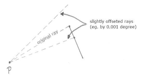
Let's see how the illumination behaves after changes:

It did not help much for the first method. We could decrease angle offset (hence increase number of rays) but the result will still be poor. On the other hand, the second method looks very smooth and accurate. From now on, we will not be talking about the first method anymore.

Visibility circle and flashlight

We may want to somehow limit player's visibility. We can achieve that by creating a clipping region of desired shape. In the demos below, I used a CanvasRenderingContext2D.clip() method.

As you might have noticed, there is no optimization whatsoever - we are still calculating all the intersection points. We will get back to it once we learn about spatial hashmaps.

What about circles?

I have rarely seen a real use-case scenario for ray casting on circles. Please treat this section as an extra where I only briefly talk about it. I will provide you with equations and basic demos, the rest is up to you.

Circle - ray intersection point

Let \(P\) be an intersection point, \(A\) a ray's anchor point, \(B\) a point on the ray, \(C\) a circle's center point and \(r\) a circle's radius. \[ \left\{\begin{align} P_x &= t(B_x - A_x) + A_x \\ P_y &= t(B_y - A_y) + A_y \\ r ^ 2 &= (P_x - C_x) ^ 2 + (P_y - C_y) ^ 2 \end{align}\right. \] Solve for \(t\): \[ \begin{align} r ^ 2 &= P_x ^ 2 - 2P_xC_x + C_x ^ 2 + P_y ^ 2 - 2P_yC_y + C_y ^ 2 \\ r ^ 2 &= (t(B_x - A_x) + A_x) ^ 2 - 2(t(B_x - A_x) + A_x)C_x + C_x ^ 2 \\ &+ (t(B_y - A_y) + A_y) ^ 2 - 2(t(B_y - A_y) + A_y)C_y + C_y ^ 2 \\ r ^ 2 &= t ^ 2 (B_x - A_x) ^ 2 + 2t(B_x - A_x)A_x + A_x ^ 2 - 2t(B_x - A_x)C_x - 2A_xC_x + C_x ^ 2 \\ &+ t ^ 2 (B_y - A_y) ^ 2 + 2t(B_y - A_y)A_y + A_y ^ 2 - 2t(B_y - A_y)C_y - 2A_yC_y + C_y ^ 2 \\ 0 &= t ^ 2 ((B_x - A_x) ^ 2 + (B_y - A_y) ^ 2) \\ &+ 2t((B_x - A_x)A_x - (B_x - A_x)C_x + (B_y - A_y)A_y - (B_y - A_y)C_y) \\ &+ A_x ^ 2 - 2A_xC_x + C_x ^ 2 + A_y ^ 2 - 2A_yC_y + C_y ^ 2 - r ^ 2 \\ 0 &= t ^ 2 ((B_x - A_x) ^ 2 + (B_y - A_y) ^ 2) \\ &+ 2t((B_x - A_x)(A_x - C_x) + (B_y - A_y)(A_y - C_y)) \\ &+ (A_x - C_x) ^ 2 + (A_y - C_y) ^ 2 - r ^ 2 \end{align} \] Solve the quadratic equation: \[ \left\{\begin{align} a &= (B_x - A_x) ^ 2 + (B_y - A_y) ^ 2 \\ b &= 2((B_x - A_x)(A_x - C_x) + (B_y - A_y)(A_y - C_y)) \\ c &= (A_x - C_x) ^ 2 + (A_y - C_y) ^ 2 - r ^ 2 \\ \Delta &= b ^ 2 - 4ac \end{align}\right. \]

• \(\Delta < 0\): ray does not intersect the circle,
• \(\Delta = 0 \): ray intersects the circle in one point (tangent),
• \(\Delta > 0 \): ray intersects the circle in two points.

Casting rays on circles

We need to find two tangent lines to a given circle passing through a ray anchor point.
Let \(P_i\) be tangent points, \(A\) a ray's anchor point, \(C\) a circle's center point and \(r\) a circle's radius.
We will also be moving all points using translation vector \(\overrightarrow{v} = (-C_x, -C_y)\): \(X^\prime = X + \overrightarrow{v}\), so the circle's center is at \((0,0)\).

From the circle equation: \[ P_x ^ {\prime ^ 2} + P_y ^ {\prime ^ 2} = r ^ 2 \] From the perpendicular line to the circle's radius: \[ \begin{align} & \tfrac{P_y ^ \prime}{P_x ^ \prime} = - \tfrac{1}{\tfrac{P_y ^ \prime - A_y ^ \prime}{P_x ^ \prime - A_x ^ \prime}} \\ & \tfrac{P_y ^ \prime}{P_x ^ \prime} = - \tfrac{P_x ^ \prime - A_x ^ \prime}{P_y ^ \prime - A_y ^ \prime} \\ & - P_y ^ {\prime ^ 2} + P_y ^ \prime A_y ^ \prime = P_x ^ {\prime ^ 2} - P_x ^ \prime A_x ^ \prime \\ & P_x ^ {\prime ^ 2} + P_y ^ {\prime ^ 2} = P_x ^ \prime A_x ^ \prime + P_y ^ \prime A_y ^ \prime \end{align} \] Solve the equation system: \[ \left\{\begin{align} & P_x ^ {\prime ^ 2} + P_y ^ {\prime ^ 2} = r ^ 2 \\ & P_x ^ {\prime ^ 2} + P_y ^ {\prime ^ 2} = P_x ^ \prime A_x ^ \prime + P_y ^ \prime A_y ^ \prime \end{align}\right. \] \[ \begin{align} & r ^ 2 = P_x ^ \prime A_x ^ \prime + P_y ^ \prime A_y ^ \prime \\ & P_x ^ \prime = \tfrac{r ^ 2 - P_y ^ \prime A_y ^ \prime }{A_x ^ \prime} \text{, where } A_x ^ \prime \neq 0 \end{align} \] Substitute \(P_x ^ \prime\) into the first equation: \[ \begin{align} & (\tfrac{r ^ 2 - P_y ^ \prime A_y ^ \prime }{A_x ^ \prime}) ^ 2 + P_y ^ {\prime ^ 2} = r ^ 2 \\ & \tfrac{r ^ 4 - 2 r ^ 2 P_y ^ \prime A_y ^ \prime + (P_y ^ \prime A_y ^ \prime) ^ 2}{A_x ^{\prime ^ 2}} + P_y ^ {\prime ^ 2} = r ^ 2 \\ & r ^ 4 - 2 r ^ 2 P_y ^ \prime A_y ^ \prime + (P_y ^ \prime A_y ^ \prime) ^ 2 + P_y ^ {\prime ^ 2} A_x ^{\prime ^ 2} = r ^ 2 A_x ^{\prime ^ 2} \\ & P_y ^ {\prime ^ 2} (A_x ^{\prime ^ 2} + A_y ^{\prime ^ 2}) - P_y ^ \prime 2r ^ 2 A_y ^ \prime + r ^ 4 - r ^ 2 A_x ^ {\prime ^ 2} = 0 \end{align} \] Solve the quadratic equation: \[ \left\{\begin{align} a &= A_x ^{\prime ^ 2} + A_y ^{\prime ^ 2} \\ b &= - 2r ^ 2 A_y ^ \prime \\ c &= r ^ 4 - r ^ 2 A_x ^ {\prime ^ 2} \\ \Delta &= b ^ 2 - 4ac \end{align}\right. \]

• \(\Delta < 0\): there are no tangent points (ray's anchor point is in the circle),
• \(\Delta = 0 \): there is only one tangent point (ray's anchor point),
• \(\Delta > 0 \): there are two tangent points.

There is still one issue - it will not work if \(A_x ^ \prime = 0\).
Take a closer look at the following equation: \(r ^ 2 = P_x ^ \prime A_x ^ \prime + P_y ^ \prime A_y ^ \prime\).
If \(A_x ^ \prime = 0\), the equation becomes: \(r ^ 2 = P_y ^ \prime A_y ^ \prime\) - we cannot substitute \(P_x ^ \prime\) anymore.
Here are the steps for solving the equation system once that happens:

Solve the equation system: \[ \left\{\begin{align} & P_x ^ {\prime ^ 2} + P_y ^ {\prime ^ 2} = r ^ 2 \\ & P_x ^ {\prime ^ 2} + P_y ^ {\prime ^ 2} = P_x ^ \prime A_x ^ \prime + P_y ^ \prime A_y ^ \prime \\ & A_x ^ \prime = 0 \end{align}\right. \] \[ \begin{align} & r ^ 2 = P_y ^ \prime A_y ^ \prime \\ & P_y ^ \prime = \tfrac{r ^ 2}{A_y ^ \prime} \text{, where } A_y ^ \prime \neq 0 \end{align} \] Substitute \(P_y ^ \prime\) into the first equation: \[ \begin{align} & P_x ^ {\prime ^ 2} + (\tfrac{r ^ 2}{A_y ^ \prime}) ^ 2 = r ^ 2 \\ & P_x ^ {\prime ^ 2} + \tfrac{r ^ 4}{A_y ^ {\prime ^ 2}} = r ^ 2 \\ & P_x ^ {\prime ^ 2} A_y ^ {\prime ^ 2} + r ^ 4 = r ^ 2 A_y ^ {\prime ^ 2} \\ & P_x ^ {\prime ^ 2} A_y ^ {\prime ^ 2} + r ^ 4 - r ^ 2 A_y ^ {\prime ^ 2} = 0 \end{align} \] Solve the quadratic equation: \[ \left\{\begin{align} a &= A_y ^ {\prime ^ 2} \\ b &= 0 \\ c &= r ^ 4 - r ^ 2 A_y ^ {\prime ^ 2} \\ \Delta &= b ^ 2 - 4ac \end{align}\right. \]

• \(\Delta < 0\): there are no tangent points (ray's anchor point is in the circle),
• \(\Delta = 0 \): there is only one tangent point (ray's anchor point),
• \(\Delta > 0 \): there are two tangent points.

Note that we can do the same for \(A_y ^ \prime = 0\), however, it is optional.
If \(A_x ^ \prime = A_y ^ \prime = 0\), there are no solutions.

Few optimization techniques

In this section, we will discuss the usage of spatial hashmaps and modified Bresenham's line algorithm. I will not go into implementation details as they are commonly available on the Internet. I will, however, provide you with some demos to try these out and come up with your own ideas on where to use them.

Spatial hashmaps

Currently, we are drawing all polygons and calculating all intersection points, but it is pretty much useless. In most cases, our play area will be much bigger than the viewport. By using spatial hashmaps, we can quickly determine which polygons are visible to the player and perform adequate calculations.

Basically, we want to divide the play area into smaller cells (of predefined size). Each cell consists of a list containing our shapes (most likely line-segments). If a single shape spans across multiple cells, it will be included in all of them.

The name of this technique suggests using hashmaps (eg. cells would be named something like X+":"+Y), but in our case, using a simple 2D array might be more desired.

Here is a simple demo showing how it might work:

We can use them for viewports as mentioned previously, and also visibility circles and flashlights.

Bresenham-based supercover line algorithm

Well, it is high time we did something with finding the closest intersection points. Using spatial hashmaps and modified Bresenham's line algorithm, we can traverse the grid in an efficient manner making as few checks as required. The algorithm should stop when the first cell with an intersection point is found.

You can read more about Bresenham's line algorithm here, and its modified version here.

Everything has an end

Sorry, unfortunately, I mean this article and not rays.

I think I have covered everything to help you get started. I will try my best to expand it in the future if I spot something needing an additional explanation. I have also created a little cheatsheet for you to quickly recap some of the topics and derived formulas.

If you enjoyed the read be sure to star and watch this repository on GitHub. You might also want to follow me for more content like that in the future. Also do not forget to create an issue if one of the topics seems to be poorly explained or you have other suggestions.

Stay tuned for more!